Stability
NSC 9
Technical Digest 2019
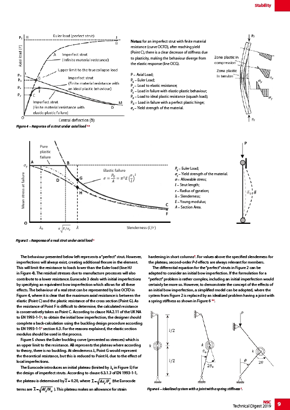
Notes: for an imperfect strut with finite material
resistance (curve OCFD), after reaching yield
(Point C), there is a clear decrease of stiffness due
to plasticity, making the behaviour diverge from
the elastic response (line OCG).
P – Axial Load;
PE – Euler Load;
Py – Load to elastic resistance;
PF – Load in failure with elastic-plastic behaviour;
PP – Load to ideal plastic resistance (squash load);
PG – Load in failure with a perfect plastic hinge;
σy – Yield strength of the material.
The behaviour presented below left represents a “perfect” strut. However,
imperfections will always exist, creating additional flexure in the element.
This will limit the resistance to loads lower than the Euler load (line HJ
in Figure 4). The residual stresses due to manufacture processes will also
contribute to a lower resistance. Eurocode 3 deals with initial imperfections
by specifying an equivalent bow imperfection which allows for all these
effects. The behaviour of a real strut can be represented by line OCFD in
Figure 4, where it is clear that the maximum axial resistance is between the
elastic (Point C) and the plastic resistance of the cross section (Point G). As
the resistance of Point F is difficult to determine, the calculated resistance
is conservatively taken as Point C. According to clause NA.2.11 of the UK NA
to EN 1993-1-13, to obtain the initial bow imperfection, the designer should
complete a back-calculation using the buckling design procedure according
to EN 1993-1-14 section 6.3. For the reasons explained, the elastic section
modulus should be used in the process.
Figure 5 shows the Euler buckling curve (presented as stresses) which is
an upper limit to the resistance. AB represents the plateau where according
to theory, there is no buckling. At slenderness λ, Point G would represent
the theoretical resistance, but this is reduced to Point H, due to the effect of
local imperfections.
The Eurocode introduces an initial plateau (limited by λ0 in Figure 5) for
the design of imperfect struts. According to clause 6.3.1.3 of EN 1993-1-1,
the plateau is determined by λ = 0.20, where
= Ay /Pcr
(the Eurocode
terms are = Afy /Ncr ). This plateau makes an allowance for strain
hardening in short columns6. For values above the specified slenderness for
the plateau, second-order P-δ effects are always relevant for members.
The differential equation for the “perfect” struts in Figure 2 can be
adapted to consider an initial bow imperfection. If the formulation for a
“perfect” problem is rather complex, including an initial imperfection would
certainly be more so. However, to demonstrate the concept of the effects of
an initial bow imperfection, a simplified model can be adopted, where the
system from Figure 2 is replaced by an idealized problem having a joint with
a spring stiffness as shown in Figure 6 2,6.
Figure 4 – Response of a strut under axial load 5.6
Figure 5 – Response of a real strut under axial load 5
PE – Euler Load;
σy – Yield strength of the material.
σ – Allowable stress;
l – Strut length;
r – Radius of gyration;
λ – Slenderness;
E – Young modulus;
A – Section Area.
Figure 6 – Idealized system with a joint with a spring stiffness 2.