Stability
Assuming that the upper and lower bars have an initial rotation “θ0”, with
zero rotation of the spring, and an axial load is applied, the rotation
increases to θ, and the moment on the spring becomes Mspring = k·2(θ - θ0),
where k is the (elastic) spring stiffness. The equilibrium in the deformed
shape leads to the following expression: Pθ l ⁄ 2 = Mspring. From the two
previous expressions, it can be shown that P = 4k
10 NSC
1
1- ( ) , where μ = Pcr ⁄ P. This is the so-called
l l
l l2 l l2
l l
Technical Digest 2019
l
- 0
( ). The critical
buckling load Pcr is for a perfectly straight member, i.e. θ0 = 0. In this case,
Pcr = 4k ⁄ l.
Therefore, P = Pcr
- 0
( ). If θ0 ≠ 0, θ would need to be infinite for P to be
equal to Pcr . This means that the imperfect column will never reach the Euler
load (this is consistent with the line OCGAB from Figure 4). The equation can
be re-written as
= 0
amplification factor. This factor allows the consideration of second order
effects by amplifying the first order effects. EN 1993-1-1 section 5.2.2
introduces this factor for frame stability in the form of
1
1-1/cr
which leads to
αcr = Pcr ⁄ P, where P is the applied load and Pcr is the elastic critical load (for a
strut, this will be Euler load). From a rigorous calculation, it can be justified
that the simplified formulation provides reasonable results for P ≤ 0.5Pcr
(αcr ≥ 2)7. EN 1993-1-1 clause 5.2.2 limits the method for frame applications
where αcr ≥ 3.
The global P-Δ effects, according to clause 5.2.1 of EN 1993-1-1 need to
be considered for the cases where the value of αcr ≤ 10 for an elastic global
analysis, and αcr ≤ 15 for a plastic global analysis. Global imperfections
for frames are defined according to EN 1993-1-1 section 5.3.2. Basically,
an initial frame rotation ϕ = h/200 (where h is the height of the frame/
structure) is recommended (Figure 1), although the value can be reduced
based on the number of columns and height of the frame. If the applied
horizontal loads in the frame are more than 15% of the vertical loads, clause
5.3.2 of EN 1993-1-1 allows the global imperfections to be neglected. In this
circumstance, the effects of global imperfections are small compared to that
of the applied horizontal loads.
To assess global instability in a structure, the problem is often addressed
using the Finite Element Method. In simple terms, the stiffness of a beam
element is reduced based on the level of axial force. The method leads to
a stiffness matrix Kt for the total structure, where the critical factor αcr is
obtained by solving the determinant |Kt| = 0. Different buckling modes
can be found (eigenvalues). For global stability, local modes (related to
individual members) are ignored. The exact answer for the problem is
complex, leading to the implementation of simplified approaches. The exact
answer for a simple beam with no axial or shear deformation is presented
in Figure 7. The terms in the matrix depend on the stability functions ϕi.
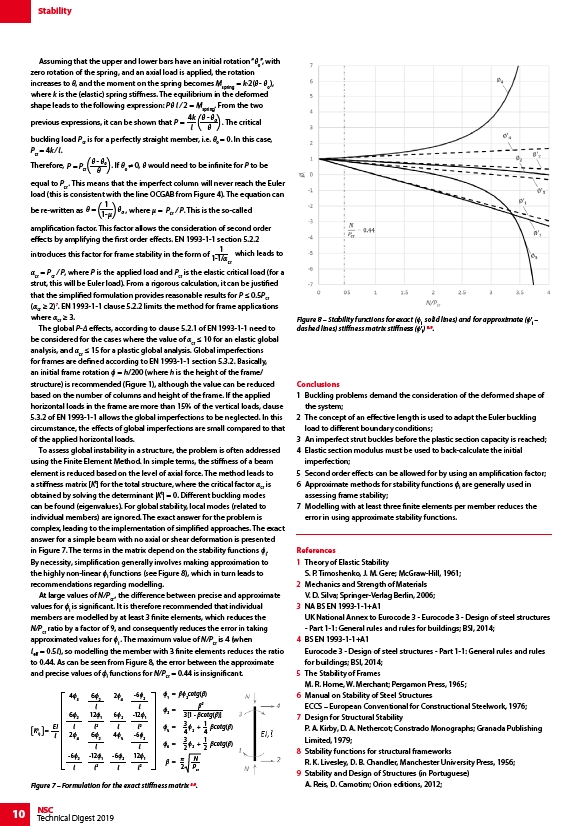
By necessity, simplification generally involves making approximation to
the highly non-linear ϕi functions (see Figure 8), which in turn leads to
recommendations regarding modelling.
At large values of N/Pcr , the difference between precise and approximate
values for ϕi is significant. It is therefore recommended that individual
members are modelled by at least 3 finite elements, which reduces the
N/Pcr ratio by a factor of 9, and consequently reduces the error in taking
approximated values for ϕi . The maximum value of N/Pcr is 4 (when
leff = 0.5l), so modelling the member with 3 finite elements reduces the ratio
to 0.44. As can be seen from Figure 8, the error between the approximate
and precise values of ϕi functions for N/Pcr = 0.44 is insignificant.
Conclusions
1 Buckling problems demand the consideration of the deformed shape of
the system;
2 The concept of an effective length is used to adapt the Euler buckling
load to different boundary conditions;
3 An imperfect strut buckles before the plastic section capacity is reached;
4 Elastic section modulus must be used to back-calculate the initial
imperfection;
5 Second order effects can be allowed for by using an amplification factor;
6 Approximate methods for stability functions ϕi are generally used in
assessing frame stability;
7 Modelling with at least three finite elements per member reduces the
error in using approximate stability functions.
References
1 Theory of Elastic Stability
S. P. Timoshenko, J. M. Gere; McGraw-Hill, 1961;
2 Mechanics and Strength of Materials
V. D. Silva; Springer-Verlag Berlin, 2006;
3 NA BS EN 1993-1-1+A1
UK National Annex to Eurocode 3 - Eurocode 3 - Design of steel structures
- Part 1-1: General rules and rules for buildings; BSI, 2014;
4 BS EN 1993-1-1+A1
Eurocode 3 - Design of steel structures - Part 1-1: General rules and rules
for buildings; BSI, 2014;
5 The Stability of Frames
M. R. Horne, W. Merchant; Pergamon Press, 1965;
6 Manual on Stability of Steel Structures
ECCS – European Conventional for Constructional Steelwork, 1976;
7 Design for Structural Stability
P. A. Kirby, D. A. Nethercot; Constrado Monographs; Granada Publishing
Limited, 1979;
8 Stability functions for structural frameworks
R. K. Livesley, D. B. Chandler, Manchester University Press, 1956;
9 Stability and Design of Structures (in Portuguese)
A. Reis, D. Camotim; Orion editions, 2012;
Kt
ij = EI
l
43 62 24
-62
62 62 121 -121
43 62 24 -62
-62 -121 -62 121
l l2 l l2
1 = 2cotg()
2 = 2
31 - cotg()
3 = 34
2 + 14
cotg()
4 = 32
2 + 12
cotg()
= 2
N
Pcr
Figure 7 – Formulation for the exact stiffness matrix 8,9.
Figure 8 – Stability functions for exact (ϕi solid lines) and for approximate (ϕ'i –
dashed lines) stiffness matrix stiffness (ϕ'i) 8,9.