Stability
Stability and second order
effects on steel structures:
Part 1: fundamental behaviour
Ricardo Pimentel of the SCI introduces the topics of buckling phenomenon, second order effects
and the approximate methods to allow for those effects. In part 2, the various methods will be
compared to the results from a rigorous numerical analysis.
When a structure is loaded, deformation occurs, and the internal forces
within the structure are modified. If at some point an increase of load (and
deflection) does not modify the internal forces, the structure becomes
unstable (only considering elastic buckling). In a perfect structure, a
theoretical sudden instability exists when the applied loads reach a critical
load. However, because real structures are always imperfect, the so-called
sudden instability does not exist – an initial bow imperfection in a strut
will increase as the applied load increases. When the applied load becomes
closer to the theoretical critical value, the deformation increases rapidly.
This leads to the following conclusions: (i) when loaded, a strut tends to
diverge from its initial position “guided” by the initial bow imperfection;
(ii) the magnitude of the initial bow imperfection will have influence in
the critical load of the strut; (iii) the applied load will have impact on the
deformed shape, which in turn will influence the buckling resistance of the
member.
From the concepts explained above, the assessment of instability
problems must consider the effects of the deformations due to the applied
loads. Even for the theoretically perfect structures, the prediction of the
load that leads to sudden instability requires the assumption of a deformed
shape of the system. To address the problem, taking the frame in Figure 1 as
example, two types of effects are important:
(i) P-δ effects, which are related to deformations within the length of
(ii) P-Δ effects, which are related to movement of nodes.
The impact of the P-δ and P-Δ effects is to change the forces and
deflections within the structure. These are second order effects, not
accounted for in a usual first order analysis. Second order effects may
be accounted for by a geometric non-linear analysis or by approximate
modifications of a first order analysis. A second order analysis can be
done through a series of first order analyses, applying the load in small
increments, but for each increment, the deformed shape of the structure is
considered.
For an idealized “perfect” pin-ended strut (Figure 2), the theoretical
8 NSC
members, and
Technical Digest 2019
critical load that leads to a sudden instability of the system can be obtained
by solving a second order differential equation1. In the process, the
displacement “y” along “z” is established using a sinusoidal function, which
later leads to the following definition:
P = n22EI
l2
where n=1,2,3…
The load P is the Euler buckling load. It is clear that there are many
possible values for P with different value of “n” leading to different buckling
mode shapes. These modes are usually called eigenvalues. The minimum
value of P (n=1), represents the critical load of the strut (Pcr), which means
that the first eigenvalue of the system will represent the critical buckling
mode shape.
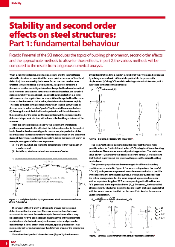
The governing equation can be re-arranged for different boundary
conditions as presented in Figure 3. For some configurations (such as “a”,
“b” or “c”), with geometric/symmetric considerations a solution is possible
without solving the differential equation. For example “a”, it is clear that
the critical configuration has the same shape of a pin-ended member
with an equivalent length of 2l. The corresponding critical load for case
“a” is presented in the expression below (Pcr,a ). The term leff is the so-called
effective length, which may be defined as the length that a pin-ended strut
with the same cross-section that has the same Euler load as the member
under consideration.
Pcr,a = n22EI
2l2 or = n22EI
leff
2
,therefore leff=2l
Figure 1 – Local (δ) and global (Δ) displacements which produce second order
effects P-δ and P-Δ.
Figure 2 – Buckling modes for a pin-ended strut2.
leff,a = 2l
leff,b = l
leff,c = 0.5l
leff,d ≈ 0.7l
Figure 3 – Effective length for struts with different boundary conditions2.