Technical
NSC 23
March 19
eigenvalues. The minimum value of P (n=1), represents the critical
load of the strut (Pcr), which means that the first eigenvalue of the
system will represent the critical buckling mode shape.
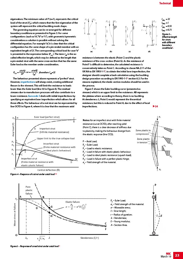
The governing equation can be re-arranged for different
boundary conditions as presented in Figure 3. For some
configurations (such as “a”, “b” or “c”), with geometric/symmetric
considerations a solution is possible without solving the
differential equation. For example “a”, it is clear that the critical
configuration has the same shape of a pin-ended member with an
equivalent length of 2l. The corresponding critical load for case “a”
is presented in the expression below (Pcr,a ). The term leff is the socalled
effective length, which may be defined as the length that
a pin-ended strut with the same cross-section that has the same
Euler load as the member under consideration.
2l2 or = n22EI
Pcr,a = n22EI
leff
2
,therefore leff=2l
The behaviour presented above represents a “perfect” strut.
However, imperfections will always exist, creating additional
flexure in the element. This will limit the resistance to loads
lower than the Euler load (line HJ in Figure 4). The residual
stresses due to manufacture processes will also contribute to a
lower resistance. Eurocode 3 deals with initial imperfections by
specifying an equivalent bow imperfection which allows for all
these effects. The behaviour of a real strut can be represented by
line OCFD in Figure 4, where it is clear that the maximum axial
(a) (b) (c) (d)
resistance is between the elastic (Point C) and the plastic
resistance of the cross section (Point G). As the resistance of
Point F is difficult to determine, the calculated resistance is
conservatively taken as Point C. According to clause NA.2.11 of the
UK NA to EN 1993-1-13, to obtain the initial bow imperfection, the
designer should complete a back-calculation using the buckling
design procedure according to EN 1993-1-14 section 6.3. For the
reasons explained, the elastic section modulus should be used in
the process.
Figure 5 shows the Euler buckling curve (presented as
stresses) which is an upper limit to the resistance. AB represents
the plateau where according to theory, there is no buckling.
At slenderness λ, Point G would represent the theoretical
resistance, but this is reduced to Point H, due to the effect of local
imperfections. 24
leff,a = 2l
leff,b = l
leff,c = 0.5l
leff,d ≈ 0.7l
Figure 3 –
Effective length
for struts
with different
boundary
conditions2.
Notes: for an imperfect strut with finite material
resistance (curve OCFD), after reaching yield
(Point C), there is a clear decrease of stiffness due
to plasticity, making the behaviour diverge from
the elastic response (line OCG).
P – Axial Load;
PE – Euler Load;
Py – Load to elastic resistance;
PF – Load in failure with elastic-plastic behaviour;
PP – Load to ideal plastic resistance (squash load);
PG – Load in failure with a perfect plastic hinge;
σy – Yield strength of the material.
Figure 4 – Response of a strut under axial load 5.6
Figure 5 – Response of a real strut under axial load 5
PE – Euler Load;
σy – Yield strength of the material.
σ – Allowable stress;
l – Strut length;
r – Radius of gyration;
λ – Slenderness;
E – Young modulus;
A – Section Area.
/Allowing_for_the_effects_of_deformed_frame_geometry
/Design_codes_and_standards#Eurocode_3_-_Steel_structures