Technical
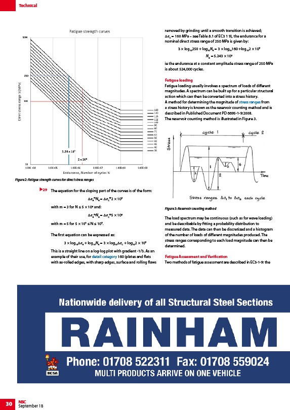
Figure 2: Fatigue strength curves for direct stress ranges
30 NSC
September 18
The equation for the sloping part of the curves is of the form:
ΔσR
mNR = ΔσC
m2 × 106
with m = 3 for N ≤ 5 × 10⁶ and:
ΔσR
mNR = ΔσC
m5 × 106
with m = 5 for 5 × 10⁶ ≤ N ≤ 108.
The first equation can be expressed as:
3 × log10ΔσR + log10NR = 3 × log10ΔσC + log102 × 106
This is a straight line on a log-log plot with gradient -1/3. As an
example of their use, for detail category 160 (plates and flats
with as-rolled edges, with sharp edges, surface and rolling flaws
removed by grinding until a smooth transition is achieved;
ΔσC = 160 MPa – see Table 8.1 of EC3 1 9), the endurance for a
nominal direct stress range of 250 MPa is given by:
3 × log10250 + log10NR = 3 × log10160 +log102 × 106
NR = 5.243 × 10⁵
ie the endurance at a constant amplitude stress range of 250 MPa
is about 524,000 cycles.
Fatigue loading
Fatigue loading usually involves a spectrum of loads of different
magnitudes. A spectrum can be built up for a particular structural
action which can then be converted into a stress history.
A method for determining the magnitude of stress ranges from
a stress history is known as the reservoir counting method and is
described in Published Document PD 6695-1-9:2008.
The reservoir counting method is illustrated in Figure 3.
The load spectrum may be continuous (such as for wave loading)
and be describable by fitting a probability distribution to
measured data. The data can then be discretized and a histogram
of the number of loads of different magnitudes produced. The
stress ranges corresponding to each load magnitude can then be
determined.
Fatigue Assessment and Verification
Two methods of fatigue assessment are described in EC3-1-9: the
29
Figure 3: Reservoir counting method
/Fatigue_design_of_bridges#Detail_categories
/Fatigue_design_of_bridges#Effects_of_varied_stress_ranges